Lunar Lander

Problem Description

An agent needs to be trained to successfully land the ‘Lunar Lander’ implemented in OpenAI gym. The Lunar-Lander has a 4 dimensional discrete action space:  go left, right, do nothing and fire the main engine. It has an 8 dimensional state space, 6 of them being continuous and 2 of them being discrete. 

With traditional Q-learning, it will be difficult to build the Q-table for high-dimensional continuous state/action spaces. Thus to solve this Lunar-Landing problem, a DQN with a separate Q-network[1] is experimented. Instead of using a Q-table, a 3 layer fully connected neural network is used to estimate the Q values.  After 2000 episodes of training, the average reward of the past 100 episode can reach ~250 points.

Training Algorithm

The training process can be summarized in the steps below:

1) The agent starts with two neural networks (the main and the target) and initialize them with random weights. Then, it will run 2000 episodes to learn about the environment.

2) During each step of any episodes, the agent acts based on an epsilon-greedy policy. A random number between 0 and 1 is generated. If it’s smaller than epsilon, then it will act randomly to explore the environment. Otherwise it will choose the best option based on the Q-values given by the main neural network.

The epsilon value will decay over time, that is, at the end of each episode it will be multiplied by a decay factor (<1), which means that it will explore the environment more at the beginning of the episodes, then gradually rely more on its own experience. A minimum epsilon value of 0.01 is applied to keep the agent doing minimum exploration.

3) After the action, an experience tuple (current_state, action, reward, next_state) can be generated and is added to the replay memory. The replay memory is implemented as a fixed size FIFO container. If the memory is full, then the oldest experience tuple will be removed.
Then the main_network will be trained on a batch of data randomly sampled from the replay memory. 

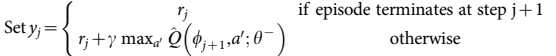
4) During training, the input data (X) are the current_states in the experience tuples from the sampled batch data, while the output date (Y) will be generated as shown in the equation below[1], in which rj is the reward in the tuple, and Q-hat term is the Q values predicted by the target network on the next_states. 

5) A counter is used to calculate the number of trainings launched on the main_network. Once it exceeds a certain threshold, the target network will be updated to be the same as the main_network, and the counter will be reset to zero.

Hyper-Parameters
Learning Rate

Fig2  Average reward over the most recent 100 episodes, with two layer network of size 256, lambda=0.99, epsilon=1, epsilon decay=0.999

Figure 2 shows a comparison of the average reward of the recent 100 episodes, with differnent learning rates applied - 0.0001, 0.01 and 0.1. When learning rate is 0.0001, the reward can reach ~150 after 1500 episodes. However the other two learning rates perform badly. 

Higher learning rates indicate larger movements of the weights in the direction of negative gradient during training. When the learning rate is too high (0.1 and 0.01 in this case), the weights can move too far and oscillating around the optimum point. However higher learning rates helps the agent to avoid stucking in a local minimum.

Lower learning rates, on the other hand, might get stuck in a local optimal point and cannot go out. The step sizes of the weights are too small that it cannot step out from local minimums. However small learning rates are not likely to show the oscillating behaviour around the final optimal point.

From the figure 0.0001 seems to give reasonable results, thus it is utilized for the final training of the agent.

Epsilon and Epsilon Decay Factor 

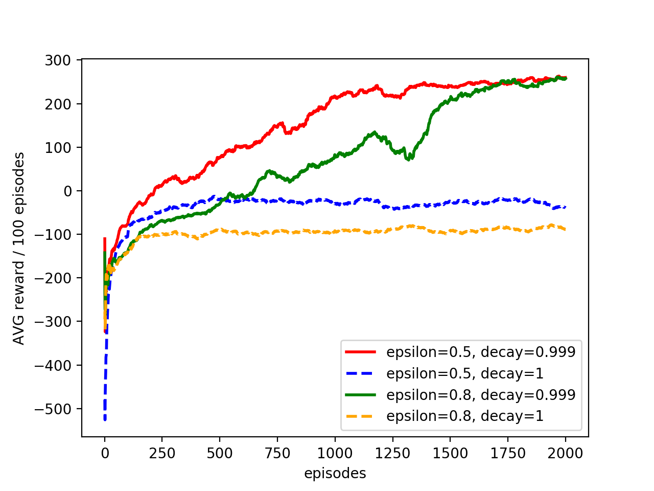
Fig3  Avg reward over the most recent 100 episodes, with two layer network of size 256, learning rate=0.0001, gamma=0.99

Figure 3 shows the effects of the epsilon value and its decay speed. We can see that epsilon<0.5 generally performs better then 0.8, with decay rate both at 1 (no deay) and 0.999.

When decay rate =1 (no decay), the performance of the agent might is always affected by this randomness. It cannot control itself with a probability of epsilon, thus its performance is gated by this randomness of its actions.

When decay rate =0.999, on the other hand, as the agent gets more familiar with the surroundings it doesn’t need to explore that much and can rely more on its own experience. In this case it can provide a better performance. It’s interesting to see that epsilon=0.5 and 0.8 rewards converge to a similar value at 2000 episodes, which makes sense because the effective epsilon is already very small and the agent already learned enough about the environment. 

The data doesn’t show lower epsilon decay factors due to limit of time, which will be needed in future work. When the epsilon decays fast, it could be stuck to a local minimum due to the disability to explore other options. 

Discount Factor

Fig4  Average reward over the most recent 100 episodes, with two layer network of size 256, learning rate=0.0001, epsilon=1, epsilon decay=0.999

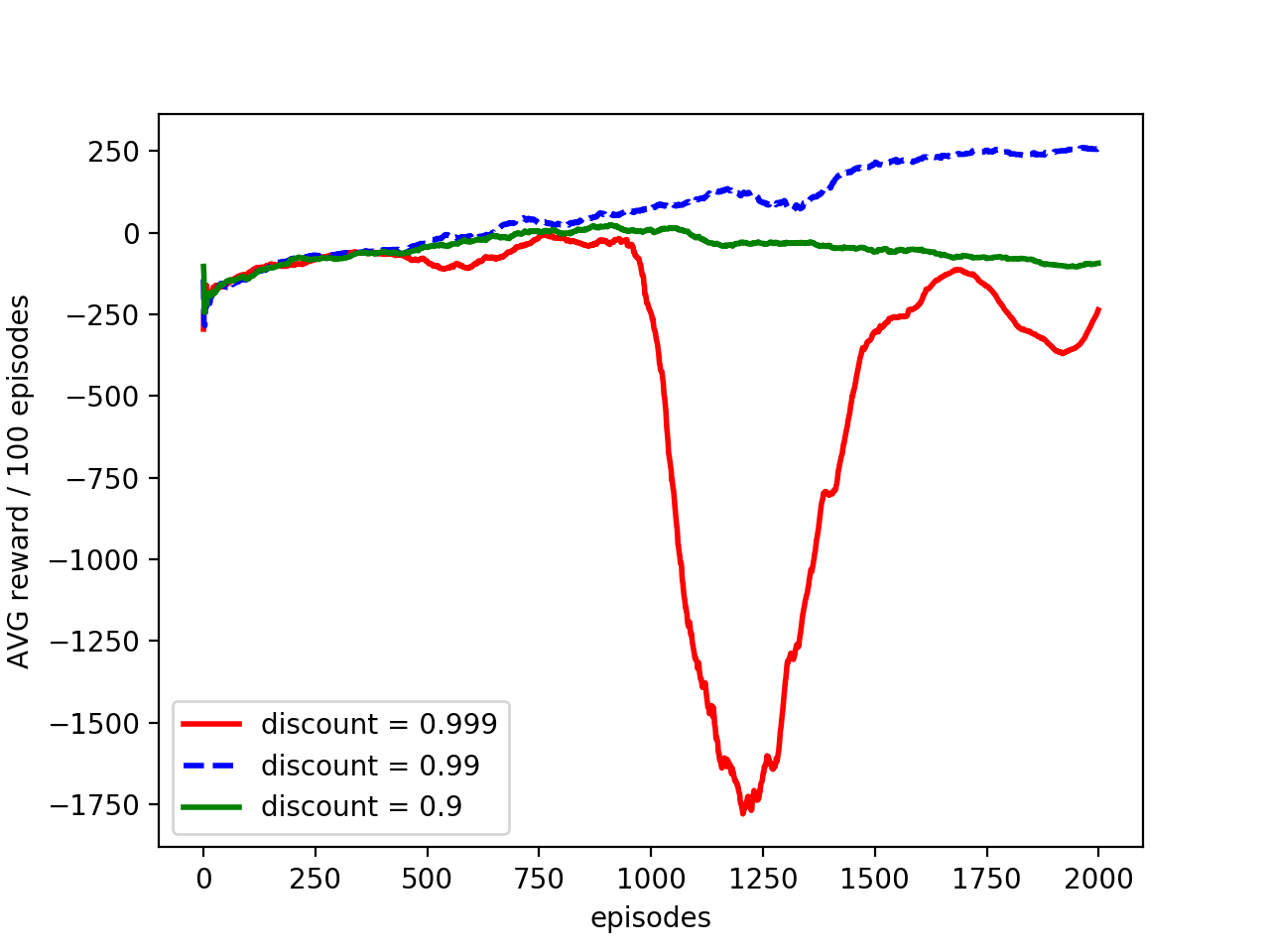
Figure 4 shows the effects of different discount factor value, on the most recent 100 episode reward during training.

From the figure we can see that when discount factor gamma rises from 0.9 to 0.99, the reward got improved. But as it goes from 0.9 to 0.999, the reward got worse. 

The discount factor determines the importance of future rewards[2]. A discount factor of ‘0’ will make the agent very short-sighted, while a factor close to 1 will make it emphasize on the long term high reward.  In another word, the gamma value tells how much the agent should rely on the future rewards.

When gamma is low, it might converge to a local sub-optimal point since it’s not seeing too much into the future. 

When gamma is too high, it will make all path to the final destination to have high Q values, discouraging the lander to approach the final destination since all actions seem to give good rewards, which could be the reason we see the <-1000 reward when gamma=0.999.

Figure 5 shows the effects of gamma combined with different epsilon & epsilon decay rate.

Comparing Fig5a & Fig5b, we see that the lower gamma value degrades performance, which is expected due to its lack of insight into the future.

                            Fig5(a)  gamma=0.9

                              Fig 5(b) gamma=0.99

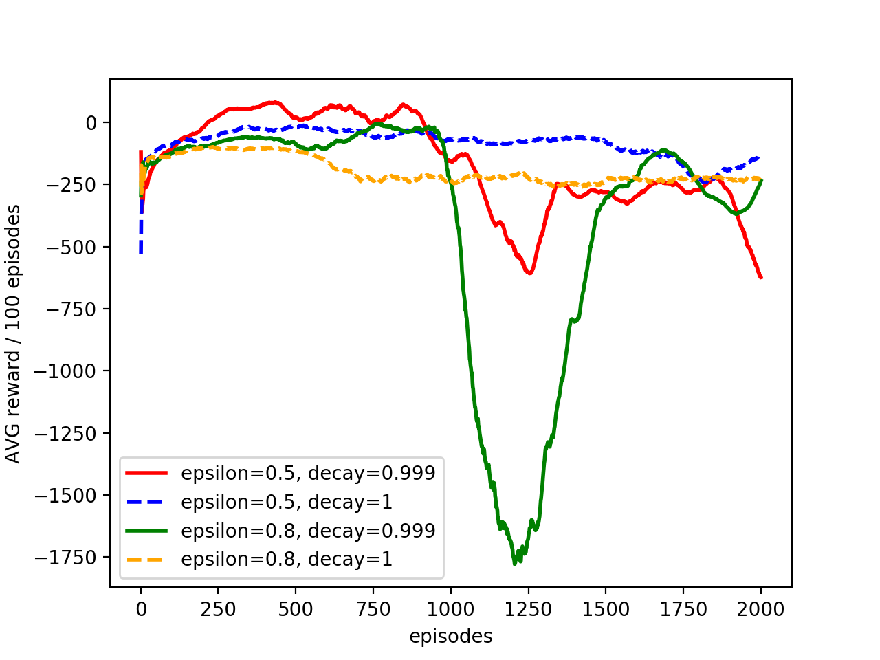
                         Fig 5(c) gamma=0.999
Fig 5 avg reward over the most recent 100 episodes, with two layer network of size 256, learning rate=0.0001

Comparing Fig5b & Fig5c, we see that the runs with decaying epsilons degrade drastically, while the runs without epsilon decay show some resistance. 

As mentioned earlier, when gamma is too high it’s difficult for the agent to differentiate between the Q values, since all Q values get high reward in the end. It’s possible that when epsilon gets smaller it fails to explore the true optimal path and thus stuck in a local optimum for a while, but managed to recover with more iterations.

When the epsilons don’t decay, the agent have the chances to explore other options, thus helping it to leave the local optimal point.

Target Network update frequency

The work in [1] introduced a target Q network to their DQN training processto reduce the likelihood of oscillation, by delaying the update of the weights in the neural network, and reported significant improvements on certain games. 

Figure 6 below shows the average reward over the most recent 100 episodes, updating the target net every 1 steps and every 100 steps for the Lunar-lander training. However no significant differences were observed. It is possible that the Lunar-lander is not complex enough to show the advantage of a second target network. It will be interesting to try apply this on other openAI problems.

Fig6  Average reward over the most recent 100 episodes, with two layer network of size 256, learning rate=0.0001, epsilon=1, epsilon decay=0.999, Updating target network ever 1 step vs every 100 steps

Final Agent

The final Agent was trained with parameters listed below:
Learning rate = 0.0001
Discount factor =0.99
Epsilon=1
Epsilon Decay factor =0.999
Neural network layer size (2 layer): 128
Replay memory size: 50000
Update target network every 100 steps.

Fig7  Average reward over the most recent 100 episodes, with two layer network of size 128 learning rate=0.0001, epsilon=1, epsilon decay=0.999, Updating target network ever 1 step vs every 100 steps

Figure7 shows the final agent’s reward during training, on each episode as well as a smoothed reward averaged over the most recent 100 episodes. After 2000 episodes it’s able to reach an average reward (for past 100 episodes) of ~250. It still gets a few runs close to 0 rewards at the very end, but overall we can see the trend gets improved.

Fig8  Reward of each episode, with two layer network of size 128, learning rate=0.0001, epsilon=1, epsilon decay=0.999, Updating target network ever 1 step vs every 100 steps

Figure 8 shows the 100 trials with the trained agent. We can see there are still a considerable amount of failures , while some of the good runs can reach ~300 points. 

Pitfalls and problems

1) At the beginning of the work I set random seed with env.seed(), np.random.seed() and random.seed(). Only until later did I realize the neural network would also need a seed to generate repeatable results.. Since I was using tensorflow, tf.random.set_seed() did the trick.

Additional works for Future

1) In this report, the minimum epsilon decay rate is 0.999. If given more time it would be interesting to see the effects if the decay rate goes lower.

2) When trying to compare the weight update frequency, this experiment didn’t show obvious advantage of using a Double DQN. However most experiments in this report are using a Double DQN agent. It will be interesting to see if the hyper-parameters have same effects on simple DQN agents, and try on some other openAI problems to see the advantages of double DQN network.

3) In this work the correlation between gamma and epsilon were studied, but it would also be interesting to see how other parameters relate to each other.

References:

[1]  V Mnih, K Kavukcuoglu, D Silver, AA Rusu, J Veness…, Human-level control through deep reinforcement learning, (2015)

[2] https://en.wikipedia.org/wiki/Q-learning

[3] https://gym.openai.com/envs/LunarLander-v2/